The United Status Census Bureau is one of the largest data collection and aggregation organizations in the United States. Their Survey and collection processes allow district lines to be drawn for voting, help local, state and municipal organizations determine how to allocate budgets, and give non-profit organizations insight into the the changing demographics of the United States. Among this incredibly valuable dataset is the American Community Survey or ACS, that collects data on race, gender, household income, employment, education, and age of citizens within each U.S. State. The ACS API or Application Program Interface is a valuable tool to collect and visualize the ACS data, without having to store it locally. The API allows you to interface with the U.S. Census Bureau portal to load the data directory into the R.
First I load I the libraries and packages necessary.
library(tidyverse)
library(tidyr)
library(ggplot2)
library(dplyr)
install.packages("broom")
library(readxl)
install.packages("stringi")
library(stringi)
install.packages("tidycensus")
library(tidycensus)
install.packages("tmap")
library(tmap)
library(tmaptools)
library(sf)
library(png)
install.packages("imager")
library(imager)
To get the load data from the ACS API. You have to apply for a U.S. Census Key. To find out more information on using the U.S. Census API go to Census API User’s Guide.
census_api_key('<api_key>', install=TRUE, overwrite=TRUE)Use the get_acs to pull the data into R.
ACS_2010 <- get_acs("state",  year=2010, variables="S1702_C02_001", output="tidy", geometry=TRUE) %>%
  select(-moe)

ACS_2011 <- get_acs("state", variables="S1702_C02_001", year=2011, output="tidy", geometry=TRUE) %>%
  select(-moe)

ACS_2012 <- get_acs("state", variables="S1702_C02_001", year=2012, output="tidy", geometry=TRUE) %>%
  select(-moe)

ACS_2013 <- get_acs("state", variables="S1702_C02_001", year=2013, output="tidy", geometry=TRUE) %>%
  select(-moe)

ACS_2014 <- get_acs("state", variables="S1702_C02_001", year=2014, output="tidy", geometry=TRUE) %>%
  select(-moe)

ACS_2015 <- get_acs("state", variables="S1702_C02_001", year=2015, output="tidy", geometry=TRUE) %>%
  select(-moe)

ACS_2016 <- get_acs("state", variables="S1702_C02_001", year=2016, output="tidy", geometry=TRUE) %>%
  select(-moe)

ACS_2017 <- get_acs("state", variables="S1702_C02_001", year=2017, output="tidy", geometry=TRUE) %>%
  select(-moe)
The variable S1702_C02_001 is the table ID for the category of data that will be loaded. The data represents housing income data. Use Tidyverse to organize and aggregate.
ACS_geo_2011 <- ACS_2011 %>%
  select('GEOID','NAME','variable','estimate','geometry') %>%
  filter(variable=='S1702_C02_001') %>%
  group_by(GEOID, NAME) %>%
  summarize(estimate = sum(estimate))

ACS_geo_2012 <- ACS_2012 %>%
  select('GEOID','NAME','variable','estimate','geometry') %>%
  filter(variable=='S1702_C02_001') %>%
  group_by(GEOID, NAME) %>%
  summarize(estimate = sum(estimate))

ACS_geo_2013 <- ACS_2013 %>%
  select('GEOID','NAME','variable','estimate','geometry') %>%
  filter(variable=='S1702_C02_001') %>%
  group_by(GEOID, NAME) %>%
  summarize(estimate = sum(estimate))

ACS_geo_2014 <- ACS_2014 %>%
  select('GEOID','NAME','variable','estimate','geometry') %>%
  filter(variable=='S1702_C02_001') %>%
  group_by(GEOID, NAME) %>%
  summarize(estimate = sum(estimate))

ACS_geo_2015 <- ACS_2015 %>%
  select('GEOID','NAME','variable','estimate','geometry') %>%
  filter(variable=='S1702_C02_001') %>%
  group_by(GEOID, NAME) %>%
  summarize(estimate = sum(estimate))

ACS_geo_2016 <- ACS_2016 %>%
  select('GEOID','NAME','variable','estimate','geometry') %>%
  filter(variable=='S1702_C02_001') %>%
  group_by(GEOID, NAME) %>%
  summarize(estimate = sum(estimate))

ACS_geo_2017 <- ACS_2017 %>%
  select('GEOID','NAME','variable','estimate','geometry') %>%
  filter(variable=='S1702_C02_001') %>%
  group_by(GEOID, NAME) %>%
  summarize(estimate = sum(estimate))
To generate the vector maps of the ACS, use tmap calls.
jpeg(file="ACS_geo_2010.jpg")
tm_shape(ACS_geo_2010) + tm_polygons("estimate") + tm_layout(title.position=c("left","top"), title="Poverty Levels in U.S. Post-Recessions", asp=1)
dev.off()

plot(load.image("ACS_geo_2010.jpg"), axes=FALSE)


tm_shape(ACS_geo_2011) + tm_polygons("estimate")

tm_shape(ACS_geo_2012) + tm_polygons("estimate")

tm_shape(ACS_geo_2013) + tm_polygons("estimate")

tm_shape(ACS_geo_2014) + tm_polygons("estimate")

tm_shape(ACS_geo_2015) + tm_polygons("estimate")

tm_shape(ACS_geo_2016) + tm_polygons("estimate")

tm_shape(ACS_geo_2017) + tm_polygons("estimate")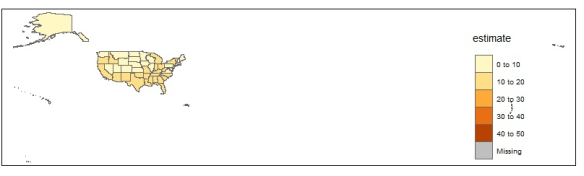
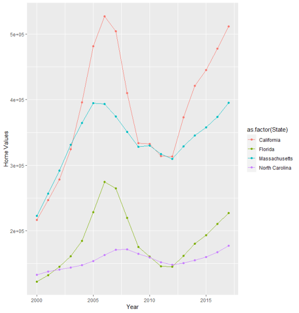
Data from the ACS portal can also be used to compare the home values by year of certain states.
ACS_Data_Housing <- ACS_Data %>%
  select('Home Values','Household Income','Bankruptcies','Percent Homeownership','Percent People in Poverty','State','Year') %>%
  filter(State %in% c("North Carolina","Massachusetts","Florida","California")) %>%
  group_by(`Year`)

ggplot(data=ACS_Data_Housing, aes(x=Year, y=`Home Values`, group=as.factor(`State`), color=as.factor(`State`))) +
   geom_line() + geom_point() +
  ylab("Home Values") +
  labs("States")