The R language has a number of machine learning libraries to help determine for both supervised and unsupervised machine learning. This includes such ML techniques such as linear and logistic regression, decision trees, random forest, generalized boosted regression modeling among others. I strongly recommend learning how these models work and how they can be used to predictive analytics.
Part of the Machine Learning process includes the following:
Sample: Create a sample set of data either through random sampling or top tier sampling. Create a test, training and validation set of data.
Explore: Use exploratory methods on the data. This includes descriptive statistics, scatter plots, histograms, etc.
Modify: Clean, prepare, impute or filter data. Perform cluster analysis, association and segmentation.
Model: Model the data using Logistic or Linear regression, Neural Networking, and Decision Trees.
Assess: Access the model by comparing it to other model types and again real data. Determine how close your model is to reality. Test the data using hypothesis testing.
When creating machine learning models for any application, it is wise to following a process flow such as the following:
In the following example, we use machine learning to determine the credit worthiness of prospective borrowers for a bank loan.
The loan data consist of the following inputs
Loan amount
Interest rate
Grade of credit
Employment length of borrower
Home ownership status
Annual Income
Age of borrower
The response variable or predictor to predict the default rate
Loan status (0 or 1).
After loading the data into R, we partition the data for training or testing sets.
loan <- read.csv("loan.csv", stringsAsFactors = TRUE)

str(loan)

## Split the data into 70% training and 30% test datasets

library(rsample)
set.seed(634)

loan_split <- initial_split(loan, prop = 0.7)

loan_training <- training(loan_split)
loan_test <- testing(loan_split)
Create a over-sample training data based on ROSE library. This checks for over-sampling of the data.
str(loan_training)

table(loan_training$loan_status)

library(ROSE)

loan_training_both <- ovun.sample(loan_status ~ ., data = loan_training, method = "both", p = 0.5)$data

table(loan_training_both$loan_status)
Build a logistic regression model and a classification tree to predict loan default.
loan_logistic <- glm(loan_status ~ . , data = loan_training_both, family = "binomial")

library(rpart)

loan_ctree <- rpart(loan_status ~ . , data = loan_training_both, method = "class")

library(rpart.plot)

rpart.plot(loan_ctree, cex=1)
Build the ensemble models (random forest, gradient boosting) to predict loan default.
loan_gbm <- gbm(loan_status ~ ., data = loan_training_both, n.trees = 200, distribution = "bernoulli")
summary(loan_gbm)
Use the ROC (receiver operating curve) and compute the AUC (area under the curve) to check the specificity and sensitivity of the models.
# Step 1. Predicting on test data

predicted_logistic <- loan_logistic %>%
  predict(newdata = loan_test, type = "response")

predicted_ctree <- loan_ctree %>%
  predict(newdata = loan_test, type = "prob")

predicted_rf <- loan_rf %>%
  predict(newdata = loan_test, type = "prob")

predicted_gbm <- loan_gbm %>%
  predict(newdata = loan_test, type = "response")

# Step 3. Create ROC and Compute AUC

library(cutpointr)

roc_logistic <- roc(loan_test, x= .fitted_logistic, class = loan_status, pos_class = 1 , neg_class = 0)
roc_ctree<- roc(loan_test, x= .fitted_ctree, class = loan_status, pos_class = 1 , neg_class = 0)
roc_rf<- roc(loan_test, x= .fitted_rf, class = loan_status, pos_class = 1 , neg_class = 0)
roc_gbm<- roc(loan_test, x= .fitted_gbm, class = loan_status, pos_class = 1 , neg_class = 0)

plot(roc_logistic) +
  geom_line(data = roc_logistic, color = "red") +
  geom_line(data = roc_ctree, color = "blue") +
  geom_line(data = roc_rf, color = "green") +
  geom_line(data = roc_gbm, color = "black")

auc(roc_logistic)
auc(roc_ctree)
auc(roc_rf)
auc(roc_gbm)
These help you compare and score which model works best for the type of data presented in the test set. When looking at the ROC chart, you can see that the gradient boost model has the best performance of all the model as it is closer to 1.00 than the other models. Classifiers that are closer to 1.00 for the top left where Sensitivity is 1.00 and Specificity is closer to 0.00 have the best performance.
Contextual text mining methods extract information from documents, live data streams and social media. In this project, thousands of tweets by users were extracted to generate sentiment analysis scores.
Sentiment analysis is a common text classification tool that analyzes streams of text data in order to ascertain the sentiment (subject context) of the text, which is typically classified as positive, negative or neutral.
In the R sentiment analysis engine, our team built, the sentiment score has a range of .-5 to 5. Numbers within this range determine the the change in sentiment.
Sentiment
Score
Negative
-5
Neutral
0
Positive
5
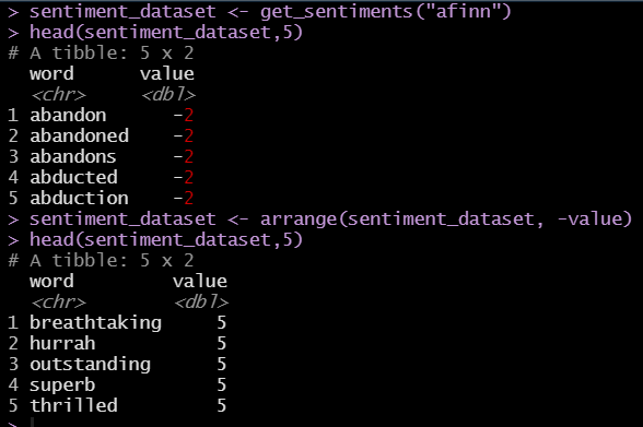
Sentiment Scores are determined by a text file of key words and scores called the AFINN lexicon. It’s a popular with simple lexicon used in sentiment analysis.
New versions of the file are released in source repositories and contains over 3,300+ words with scores associated with each word based on its level of positivity or negativity.
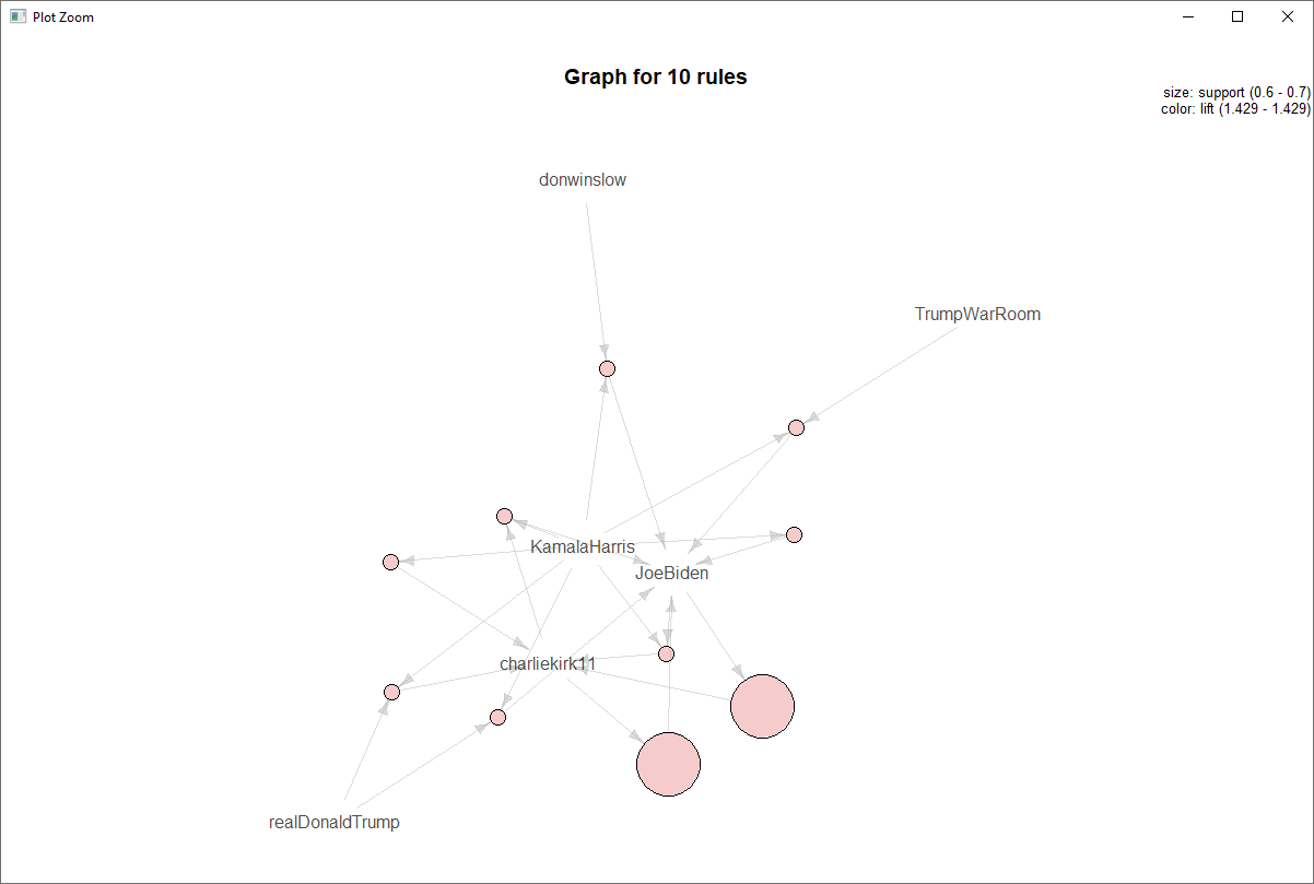
Twitter is an excellent example of sentiment analysis.
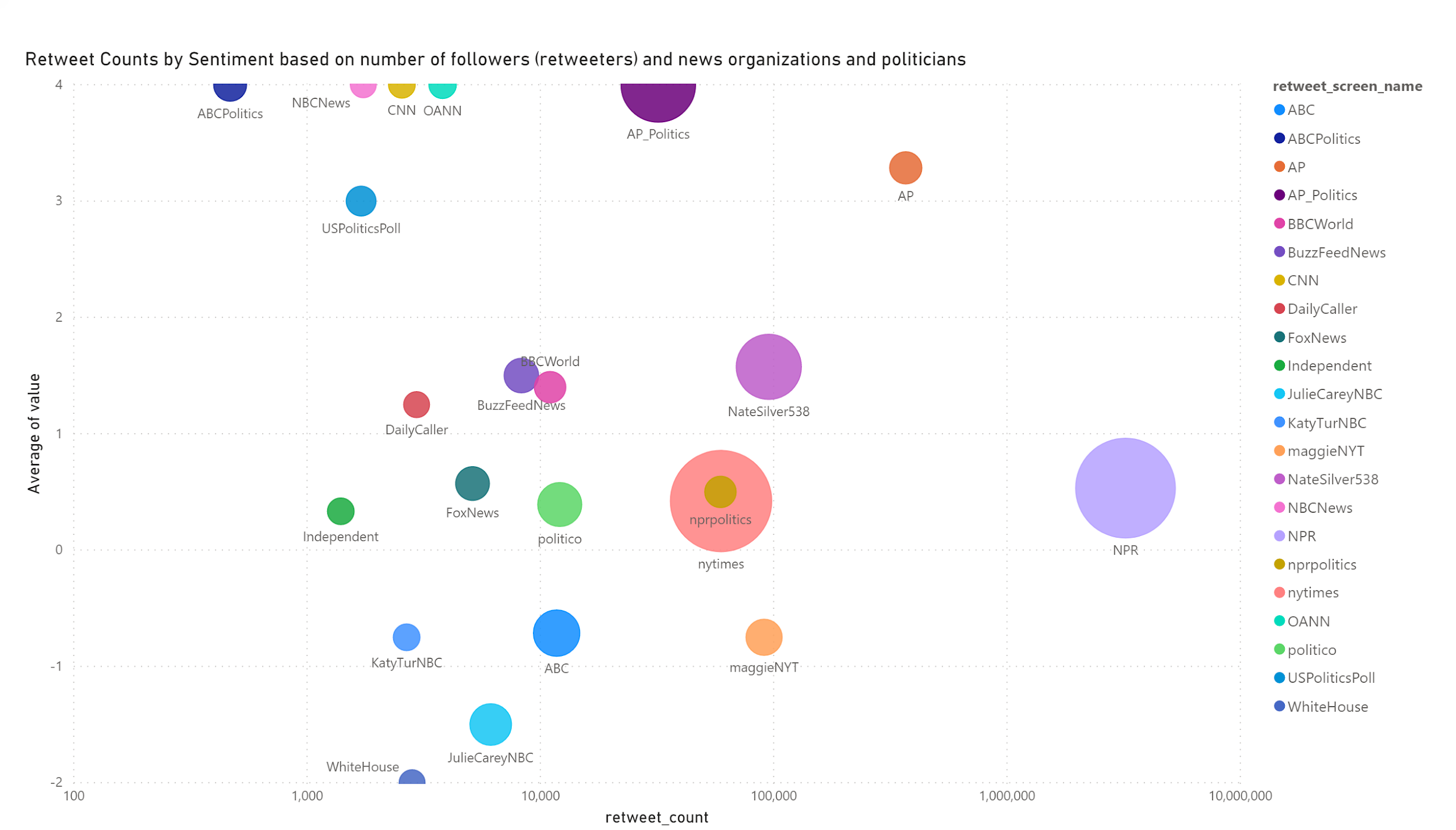
An example of exploration of the sentiment scores based on the retweets filtered on the keywords:
Trump
Biden
Republican
Democrat
Election
The data was created using a sentiment engine built in R. It is mostly based on the political climate in the United States leading up to and after the 2020 United States election.
Each bubble size represents the followers of user who’ve retweeted. The bubble size gives a sense of the influence of those users (impact). The Y-axis is the sentiment score, the X-axis represents the retweet count of the bubble name.
“Impact” is a measure of how often a twitter user is retweeted by users with high follower counts.
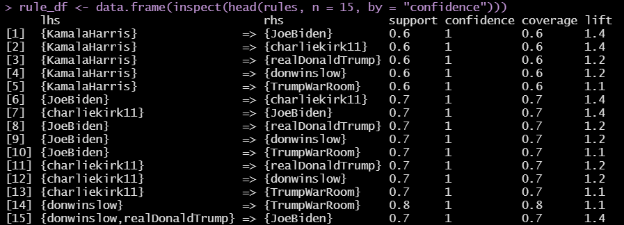
Applying the Apriori algorithm. using the single format, we assigned our transactions as the sentiment score and We assigned items_id as retweeted_screen_name.
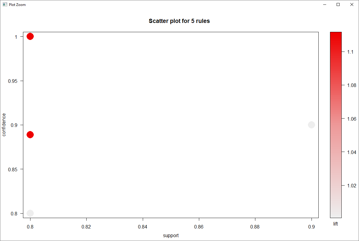
This is the measure the association between highly retweeted accounts and their associations based on sentiment scores (negative, neutral, positive). Support is the minimum support for an itemset. Minimum support was set to 0.02.
The majority of the high retweeted accounts had highly confident associations based on sentiment values. We then focused on the highest confidence associates that provided lift above 1. After removing redundancy, we were able to see the accounts where sentiment values are strongly associated between accounts.
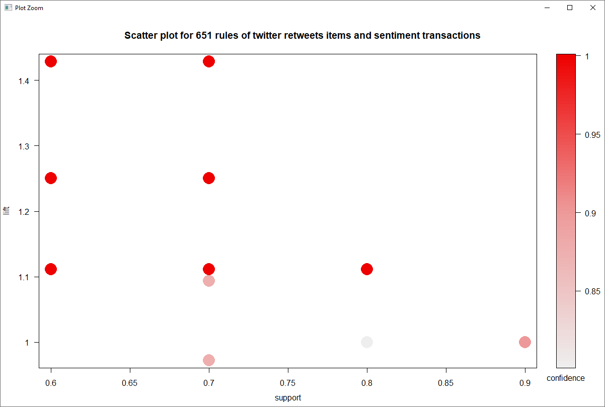
According to the scatter plot above, we see most of the rules overlap, but have very good lift due to strong associations, but also this is indicated by the limited number of transactions and redundancy in the rules.
The analysis showed a large number of redundancy, but this was mostly due to the near nominal level of sentiment values. So having high lift, a larger minimum support and .removing redundancy find the most valuable rules.
R is a great language for creating decision tree classification for a wide array of applications. Decision trees are a tree-like model in machine learning commonly used in decision analysis. The technique is commonly used in creating strategies for reaching a particular goal based on multi-dimensional datasets.
Decision trees are commonly used for applications such as determining what type of consumer is at higher risk of defaulting on a loan than borrowers of lower risk. What sort of factors impacts whether a company can retain customers, and what type of students are more at risk at dropping out and require mediation based on school attendance, grades, family structure, etc.
Below are the typically libraries for building machine learning analysis are below including decision trees, linear and logistic regression
The following code block creates regression and decision tree analysis of custom churn predictions.
# Import the customer_churn.csv and explore it.
# Drop all observations with NAs (missing values)


customers <- read.csv('customer_churn.csv')
summary(customers)
str(customers)
customers$customerID <- NULL
customers$tenure <- NULL
sapply(customers, function(x) sum(is.na(x)))
customers <- customers[complete.cases(customers),]


#===================================================================


#  Build a logistic regression model to predict customer churn by using predictor variables (You determine which ones will be included).
# Calculate the Pseudo R2 for the logistic regression.


# Build a logistic regression model to predict customer churn by using predictor variables (You determine which ones will be included).

customers <- customers %>%
 mutate(Churn=if_else(Churn=="No", 0, 1))


str(customers)

regression1 <- glm(Churn ~ Contract + MonthlyCharges + TotalCharges + TechSupport + MultipleLines + InternetService, data=customers, family="binomial")


# Calculate the Pseudo R2 for the logistic regression.


regression1 %>%
  PseudoR2()

#  Split data into 70% train and 30% test datasets.
#  Train the same logistic regression on only "train" data.

#  Split data into 70% train and 30% test datasets.


set.seed(645)

customer_split <- initial_split(customers, prop=0.7)
train_customers <- training(customer_split)
test_customers <- testing(customer_split)

# Train the same logistic regression on only "train" data.

regression_train <- glm(Churn ~ Contract + MonthlyCharges + TotalCharges + TechSupport + MultipleLines + InternetService, data=train_customers, family="binomial")
#regression_test <- glm(Churn ~ Contract + MonthlyCharges + TotalCharges + tenure + TechSupport, data=test_customers)


#  For "test" data, make prediction using the logistic regression trained in Question 2.
#  With the cutoff of 0.5, predict a binary classification ("Yes" or "No") based on the cutoff value,
#  Create a confusion matrix using the prediction result.

#. For "test" data, make prediction using the logistic regression trained in Question 2.

str(regression_train)
prediction <- regression_train %>%
  predict(newdata = test_customers, type = "response")


# With the cutoff of 0.5, predict a binary classification ("Yes" or "No") based on the cutoff value,


#train_customers <- train_customers %>%
#  mutate(Churn=if_else(Churn=="0", "No", "Yes"))
Check the sensitivity and specificity of the classification tree, we create a confusion matrix for ROC charts. ROC Charts are receiver operating characteristic curves that have the diagnostic ability of a binary classifier system as its threshold.
set.seed(1304)

train_cust_dtree_over <- ovun.sample(Churn ~., data=train_customers, method="over", p = 0.5)$data
train_cust_dtree_under <- ovun.sample(Churn ~., data=train_customers,  method="under", p=0.5)$data
train_cust_dtree_both <- ovun.sample(Churn ~., data=train_customers, method="both", p=0.5)$data

table(train_customers$Churn)
table(train_cust_dtree_over$Churn)
table(train_cust_dtree_under$Churn)
table(train_cust_dtree_both$Churn)

train_cust_dtree_over_A <- rpart(Churn ~ ., data = train_cust_dtree_over, method="class")
rpart.plot(train_cust_dtree_over_A, cex=0.8)

customers_dtree_prob <- train_cust_dtree_over_A %>%
  predict(newdata = test_customers, type = "prob")

#  Create a confusion matrix using the prediction result.


head(customers_dtree_prob)

table(customers_dtree_prob)

customers_dtree_class <- train_cust_dtree_over_A %>%
  predict(newdata = test_customers, type = "class")

table(customers_dtree_class)

test_customers <- test_customers %>%
    mutate(.fitted = customers_dtree_prob[, 2]) %>%
    mutate(predicted_class = customers_dtree_class)


confusionMatrix(as.factor(test_customers$predicted_class), as.factor(test_customers$Churn), positive = "1")
#===================================================================


#  Based on prediction results in Question 3, draw a ROC curve and calculate AUC.


roc <- roc(test_customers, x=.fitted, class=Churn, pos_class=1, neg_clas=0)

plot(roc)
auc(roc)

plot(roc) +
    geom_line(data = roc, color = "red") +
    geom_abline(slope = 1) +
    labs(title = "ROC Curve for Classification Tree")
Directions on How to Build the Predictive Model In Microsoft Azure ML
Sign in to Microsoft Azure using your login credentials in the Azure portal
Create a workspace for you to store your work
In the upper-left corner of Azure portal, select + Create a resource.
Use the search bar to type Machine Learning.
Select Machine Learning.
In the Machine Learning pane, select Create to begin.
You will provide the following information below to configure your new workspace:
Subscription – Select the Azure subscription that you would like to use.
Resource group – Create a name for your resource group which will hold resources for your Azure solution.
Workspace name – Create a unique name that identifies your workspace.
Region – select the region closest to the users to reduce latency
Storage account – created by default
Key Vault – created by default
Application insights – created by default
When you have completed configuring the workspace, select Review + Create.
Review the settings and make any additional changes or corrections. Lastly, select Create. When deployment of workspaces has completed you will see the message “Your deployment is Complete”. Please see the visual below as a reference.
To Launch your workspace, click Go to resource
Next, Click the blue Launch Studio button which is under Manage your Machine Learning Lifecycle. Now you are ready to begin!!!!
Click on Experiments in the left panel
Click on NEW in the lower left corner
Select Blank Experiment. The new experiment is created with a default name. You can change the name at the top of the page.
Upload the data above into Ml studio
Drag the datasets on to the experiment canvas. (We uploaded preprocessed data
If you would like to see what the data looks like, click on the outpost port at the bottom on the dataset and select Visualize. Given this data we are going to try and predict if there the IoT sensors have communication errors.
Next, prepare the data
Remove unnecessary columns /data
Type “Select Columns” in the Search box and select Select Columns in the Dataset module, then drag and drop it on the canvas. This allows you to exclude any columns that you do not want in the model.
Connect Select Columns in Dataset to the Data on the canvas.
Choose and Apply a Learning Algorithm
Click on Data Transformation in the left column
Next, click on the drop down Manipulation
Drag the Select Edit the Metadata (use this to change the metadata that is associated with columns inside the dataset. This changes the metadata inside Azure Machine Learning that tells the downstream components how to use the selected columns.)
Split the data
Then, click on the drop down Sample and Split.
Choose Split Data and add it to the canvas and connect it to Edit the Metadata.
Click on Split Data and find the Fraction of rows in the output dataset and set it to .80. You are splitting the data to train the model using 80% of the data and test the model using 20% of the data.
Then you train the data
Choose the drop down under Machine Learning
Choose the drop down under Initialize Model
Choose the drop down under Anomaly Detection
Click on PCA- Based Anomaly Detection and add this to the canvas and connect with the Split data.
Choose the drop down under Machine Learning
Choose the drop down under Initialize Model
Choose the drop down under Anomaly Detection
Click on One-Class Support Vector machine and add this to the canvas and connect with the Split data.
Choose the drop down under Machine Learning
Then, choose the drop down under Train
Click on Tune Model Hyperparameters and add this to the canvas and connect with the Split Data.
Choose the drop down under Machine Learning
Then, choose the drop down under Train
Click on Train Anomaly Detection Model
Then score the model
Choose the drop down under Machine Learning
Then, choose the drop down – Score
Click on Score Model
Normalize the data
Choose the drop down under Data Transformation
Then, choose the drop down under Scale and Reduce
Click on Normalize Data
Evaluate the model – this will compare the one-class SVM and PCA – based anomaly detectors.
Choose the drop down under Machine Learning
Then, choose the drop down under Evaluate
Click on Evaluate Model
Click Run at the bottom of the screen to run the experiment. Below is how the model should look. Please click on the link to use our experiment (Experiment Name: IOT Anomaly Detection) for further reference. This link requires that you have a Azure ML account. To access the gallery, click the following public link: https://gallery.cortanaintelligence.com/Experiment/IOT-Anomaly-Detection
Part two of a series of LinkedIn articles based on Cognitive Computing and Artificial Intelligence Applications
Background
Several high profile incidents of ransomware attacks have called attention to IoT networks security. An assessment of security vulnerabilities and penetration testing have become increasingly important to sufficient design. Most of this assessment and testing takes place at the software and hardware level. However, a more broad approach is vital to the security of IoT networks. The protocol and traffic analysis is of importance to structured dedicated IoT networks since communication and endpoints are tracked and managed. Understanding all the risks posed to these types of network allows for more complete risk management plan and strategy. Beside network challenges, there are challenges to scalability, operability, channels and also the information being transmitted and collected with such networks. In IoT networks, looking for vulnerabilities spans the network architecture, endpoint devices and services, where services include the hardware, software and processes that build an overall IoT architecture. Building a threat assessment or map, as part of an overall security plan, as well as, updating it on a schedule basis allows security professionals and stakeholders to manage for all possible threats to the architecture. Whenever possible, creating simulations of possible attack vectors, understanding the behavior of such attacks and then creating models will help build upon a overall security management plan.
Open ports, SQL injection flaws, unencrypted services, insecure network interfaces, buffer overflow risks, lack of firewall protocols, authorization settings, web interface insecurity are among some of the types of vulnerabilities in an IoT network and devices.
Where is the location of a impending attack? Is it occurring at the device, server or service? Is it occurring in the location where the data is stored or while the data is in transit? What type of attacks can be identified? Types of attacks include distributed denial of service, man-in-the-middle, ransomware, botnets, spoofing, account penetrations, etc.
Business Use Case
For this business use case research study, a fictional company was created. The company is a national farmland and agricultural cooperative that supplies food to local and state markets. Part of the company’s IT infrastructure is an IoT network that uses endpoint devices for monitoring and controlling temperature, humidity and moisture for the company’s large agricultural farmlands. This network has over 2000 IoT devices in operations on 800 acres. Any intrusion into the network by a rogue service or bad actor could have consequences in regards to delivering fresh produce with quality and on time. The network design in the simulation below is a concept of this agricultural network. Our team created a simulation network using Cisco Packet Tracer, a tool which allows users to create and simulate package traffic throughout a computerized network at multiple ISO levels.
Simulated data was generated for using the packet tracer simulator to track and build. In the simulation network below using multiple routers, switches, servers and IoT devices for packets such as TCP, UDP, RIPv4 and ICMP, for instance.
Network Simulation
Below is a simulation of packet routing throughout the IoT network.
Problem Statement
Our fictional company will be the basis of our team’s mock network for monitoring for intrusions and anomaly. Being a simulated IoT network, it contains only a few dozen IoT enabled sensors and devices such as sprinklers, temperature and water level sensors, and drains. Since our model will be designed for large scale IoT deployment, it will be trained on publicly available data, while the simulated data will serve as a way to score the accuracy of the model. The simulation has the ability to generate the type of threats that would create anomalies. It is important to distinguish between an attack and a known issue or event (see part one of this research for IoT communication issues). The company is aware of those miscommunications and has open work orders for them. The goal is for our model is to be able to detect an actual attack on the IP network by a bad actor. Although miscommunication is technically an anomaly, it is known by the IT staff and should not raise an alarm. Miscommunicating devices are fairly easy to detect, but to a machine learning or deep learning model, it can be a bit more tricky. Creating a security alarm for daily miscommunication issues that originate from the endpoints, would constitute a prevalence of false positives (FP) in a machine learning confusion matrix.
A running simulation
Project Significance and Implementation
In today’s age of modern technology and the internet, it is becoming increasingly more difficult to protect enterprise networks against malicious attacks. Not only are malicious actors becoming more advanced with the methodologies of their attacks, but also the number IoT devices that live and operate in a business environment is ever increasing. It needs to be a top priority for any business to create an IT business strategy that protects the company’s technical architecture systems and core intellectual property. When accessing all potential security weakness, you must decompose the network model and define trust zones within the IoT architecture.
This application was designed to use Microsoft Azure Machine Learning analyze and detect anomalies in large data sets collected from all devices on the business’ network. In an actual implementation of this application, there would be a constant data flow running through our predictive model to classify traffic as Normal, Incorrect Setup, Distributed Denial of Service (DDOS attack), Data Type Probing, Scan Attack, or Man in the Middle. Using a supervised learning method to iteratively train our model, the application would grow increasingly more cognitive, and accurate at identifying these network traffic patterns correctly. If this system were to be fully implemented, there would need to also be actions for each of these classification patterns. For instance, if the model detected a DDOS attack coming from a certain device, the application would automatically send shutdown commands to the device, thus isolating it from the network and containing the attack. When these actions occur, there would be logs taken, and notifications automatically sent to appropriate IT administrators and management teams, so that quick and effective action could be taken. Applications such as the one we have designed are already being used throughout the world by companies in all sectors. Crowdstrike for instance, is a cyber technology company that produces Information Security applications with machine learning capabilities. Cyber technology companies such as Crowdstrike have grown ever more popular over the past few years as the number of cyber attacks have increased. We have seen first hand how advanced these attacks can be with data breaches on the US Federal government, Equifax, Facebook, and more. The need for advanced information security applications is increasing daily, not just for large companies, but small- to mid-sized companies as well. While outsourcing information security is an easy choice for some companies, others may not have the budget to afford such technology. That is where our application gives an example of the low barrier to entry that can be attained when using machine learning applications, such as Microsoft Azure ML or IBM Watson. Products such as these create relatively easy interfaces for IT Security Administrators to take the action into their own hands, and design their own anomaly detection applications. In conclusion, our IOT Network Anomaly Detection Application is an example of how a company could design and implement it’s own advanced cyber security defense applications. This would better enable any company to protect it’s network devices, and intellectual property against the ever growing malicious attacks.
Methodology
For this project, our team acquired public data from Google, Kaggle and Amazon. For the IoT model, preprocessed data was selected for the anomaly detection model. Preprocessed data from the Google open data repository was collected to test and train the models. R Studio programming served as an initial data analysis and data analytics process to determine Receiver Operating Characters (ROC) and Area Under the Curve (AUC) and evaluate the sensitivity and specificity of the models for scoring the predictability of the response variables. In R, predictability was compared between with logistic regression, random forest, and gradient boosting models. In the preprocessed data, a predictor (normality) variable was used for training and testing purposes. After the initial data discovery stage, the data was processed by a machine learning model in Azure ML using support vector machine and principal component analysis pipelines for anomaly detection. The response variable has the following values:
Normal – 0
Wrong Setup – 1
DDOS – 2
Scan Attack – 4
Man in the Middle – 5
The preprocessed dataset for intrusion detection for network-based IoT devices includes ultrasonic sensors using Arduino microcontrollers and Node MCU, a low-cost open source IoT platform that can run on the ESP8266 Wi-Fi Module used to send data.
The following table represents data from the ethernet frame which is part of the TCP/IP packet that is transmitted from a source device to a destination device for network communication. The following dataset is preprocessed according to the network intrusion detection based system.
The following table represents data from the ethernet frame which is part of the TCP/IP packet that is transmitted from a source device to a destination device for network communication.
Source: Google.com
In the next article, we’ll be exploring the R code and Azure ML trained anomaly detection models in greater depth.
This is part one of a series of articles to be published on LinkedIn based on a classroom project for ISM 647: Cognitive Computing and Artificial Intelligence Applications taught by Dr. Hamid R. Nemati at the University of North Carolina at Greensboro Bryan School of Business and Economics.
The Internet of Things (IoT) continues to be one of the most innovative and exciting areas of technology in the last decade. IoT are a collection of devices that reside in the world that collect data from the environment around it or through mechanical, electrical, thermodynamic or hydrological processes. These environments could be the human body, geological areas, the atmosphere, etc. The networking of IoT devices has been more prevalent in the many industries for years including the gas, oil and utilities industry. As companies create demand for higher sample read rates of data from sensors, meters and other IoT devices and bad actors from foreign and domestic sources have become more prevalent and brazen, these networks have become vulnerable to security threats due to their increasing ubiquity and evolving role in industry. In addition to this, these networks are also prone to read rate fluctuations that can produce false positives for anomaly and intrusion detection systems when you have enterprise scale deployment of devices that are sending TCP/IP transmissions of data upstream to central office locations. This paper focuses on developing an application for anomaly detection using cognitive computing and artificial Intelligence as a way to get better anomaly and intrusion detection in enterprise scale IoT applications.
This project is to use the capabilities of automating machine learning to develop a cognitive application that addresses possible security threats in high volume IoT networks such as utilities, smart city, manufacturing networks. These are networks that have high communication read success rates with hundreds of thousands to millions of IoT sensors; however, they still may have issues such as:
Noncommunication or missing/gap communication.
Maintenance Work Orders
Alarm Events (Tamper/Power outages)
In large scale IoT networks, such interruptions are normal to business operations. Certainly, noncommunication is typically experienced because devices fail, or get swapped out due to a legitimate work order. Weather events and people, can also cause issues with the endpoint device itself, as power outages can cause connected routers to fail, and tampering with a device, such as people trying to do a hardwire by-pass or removing a meter.
The scope of this project is to build machine learning models that address IP specific attacks on the IoT network such as DDoS from within and external to the networking infrastructure. These particular models should be intelligent enough to predict network attacks (true positive) versus communication issues (true negative). Network communication typical for such an IoT network include:
Short range: Wi-Fi, Zigbee, Bluetooth, Z-ware, NFC.
Long range: 2G, 3G, 4G, LTE, 5G.
Protocols: IPv4/IPv6, SLIP, uIP, RLP, TCP/UDP.
Eventually, as such machine learning and deep learning models expand, these types of communications will also be monitored.
Scope of Project
This project will focus on complex IoT systems typical in multi-tier architectures within corporations. As part of the research into the analytical properties of IT systems, this project will focus primarily on the characteristics of operations that begin with the collection of data through transactions or data sensing, and end with storage in data warehouses, repositories, billing, auditing and other systems of record. Examples include:
Building a simulator application in Cisco Packet Tracer for a mock IoT network.
Creating a Machine Learning anomaly detection model in Azure.
Generating and collecting simulated and actual TCP/IP network traffic data from open data repositories in order to train and score the team machine learning model.
Other characteristics of the IT systems that will be researched as part of this project, include systems that preform the following:
Collect, store, aggregate and transport large data sets
Require application integration, such as web services, remote API calls, etc.
I suspect building a full-size self-driving car seems like a momentous task – and it is. But a few things we have going for us. As I stated in my previous blog, autonomous (self-driving) cars have a lot of the STEM aspects you want to instill in your child – math, science, electronics, and technology. So even if you don’t finish this, those subjects will take your child far.
A few things I would recommend is building a design for you car. The cheapest way of designing anything is using a Computer-Aided Design (CAD) software. For me, this is Autodesk® AutoCAD® 2017. It’s a great software package, but a little on the pricey side. There are also plenty of open source CAD software packages available. The nice thing about AutoCAD is that i comes with an add-on called Autodesk EAGLE, which is a electronics schematic design tool. Inevitably, there will be some electronic circuits required to build the prototype and eventually the actual car, so having an electronics design tool will be very helpful.
Autodesk EAGLE, a electronics design tool
I alluded this earlier in one of my blogs, but you will want to build a prototype that makes it easier for kids to learn about the curriculum and about the subject matter involved. A prototype has a smaller budget an can be a much smaller than the eventual final product. In my case I took apart one of my child’s toys and hooked it up to a RaspberryPi and Arduino (see Part 2 for more info).
Having a cash budget and setting design limitations on the car will take out a some of the risk of a venture such as this. For instance, our stated goal was to create a car that would not have an occupant riding inside of it, nor would it be on any public roads. This would not require us to get specific permits or spend heavily on safety features of the car. Before building anything large, my recommendation is to have the following:
A budget. My budget is going to be around $15,000 adjusted for inflation.
A goal statement or what you want to achieve that makes the project a successful learning experience.
design goals. The must haves to achieve the goal you want.
If you want to get really crazy, an actual project plan.
We actually plan to create multiple prototypes, as our skills increase, so will the quality and “coolness” of our design. This RC car we plan to use for our second prototype:
The body of the prototype II car will a Porsche. Prototype I is almost done 🙂 !
The internal frame of prototype II car. Once completed, it will have cameras, computers, and motors. There will be other devices as well to help with autonomy.
“The two biggest challenges with this project is: 1) Getting your kids more interested in the project over their video games. 2) Convincing your child’s science teacher they did most of the work for the school science fair”
Before I start delving into the technical rigors of building a self-driving car. I want to talk about kids. As parents, we want our kids to be excited about things we get excited about. When I thought up this project, I realized it was above what a fifth grader could do. A self-driving car involves a multitude of technical subjects: Advanced calculus, statistics, probability, linear algebra, deep learning, machine learning, electronics, computer science, telemetry, data science, mechanics, physics,…These are subjects kids are not expected to be good at. But, I thought to myself “It’s about the Journey…”.
As a parent, I want to expose my kids to STEM (Science, Technology, Engineering, Math). This project is STEM³, meaning, it’s several factors above what is typically taught in grade school level STEM curriculum. So how do you incorporate this into a child’s STEM education without frustrating your child and yourself in the process?
Divide things up into simpler lessons
So when my child and I started thinking about building a self-driving car, we started small. We converted a radio controlled car into a self driving robot using the following components:
Raspberry Pi 3 microcomputer.
Arduino Microcontroller
OpenCV computer vision software.
Chassis of an old RC car.
Electric 9V Motor
We then said, “What are the major components that a self-driving car would need”. What we listed were:
A Motor
Steering
A computer
A camera
Doing our research into companies like Waymo, Google, Volvo, Tesla among others who are investing millions into autonomous technology, we began learning that among these pioneering companies are a community of tinkerers who are using open source code and open hardware to build autonomous RC cars. Many of whom are blogging about it. To learn more about these communities, I recommend the blog series. Becoming Human AI.
With then focused on specific topics, that children could research and learn about.
For the Motor: Pulse Width Modification.
For the Steering: Controlling sweeper servo moters.
For the Computer: Programming Raspberry PI with Python.
For the Camera: Using OpenCV for image processing.
School Science Fair Skepticism
When we attended my child’s science fair, we had spent weeks going over Pulse Width Modification, which is a way to control an electronic motor speed and building a sweeper motor for our prototype RC autonomous car. We stuck on a Raspberry PI 3 computer which is basically a very cheep microcomputer that you can program and load up with an open source software package called OpenCV. OpenCV can detect images from a camera be recognize what that object is at least detect things in an image. When we were done our science fair project looked like this:
We spent weeks putting this together, and I made certain my child understood each component in the car and had the knowledge to talk about it. What I quickly noticed was among the baking soda volcanoes, and the dyed flower petal experiments, was a lot of skepticism that a fifth grader could put something like a “self driving robot”-thingy together.
My child put the poster together and did all the calculations as I stood by and asked “So what can you include from those findings?” The scientific method, which is the most important tool in science, was reiterated throughout the experiment:
What are observations?
What is your hypothesis?
What methodology did you use?
What is your experiment?
What were you conclusions (what did you learn)?
This is what needs to be the basis for a child’s work in STEM projects in order for him or her to learn from the successes and failures of doing science and technology.
The picture above is my child’s science fair poster. We worked pretty hard on it. But my child did all of analysis and calculations and took all of the notes and typed it up. I gave him a test to make certain that he understood everything. The goal wasn’t to win (he didn’t) it was to get him interested in science and technology and show him that there are others that are excited as well…And many people were!


![IMG_2630[1]](https://i0.wp.com/rtpopendata.com/wp-content/uploads/2019/08/img_26301.jpg?resize=584%2C438&ssl=1)
![IMG_2635[1]](https://i0.wp.com/rtpopendata.com/wp-content/uploads/2019/08/img_26351.jpg?resize=584%2C438&ssl=1)